Tip
Run this notebook online: ![]() . Note that the set up can take a while, as all the dependencies must be installed first.
. Note that the set up can take a while, as all the dependencies must be installed first.
1. Manipulating a trajectory
This notebook shows how to read and manipulate the trajectories in which the system’s configurations are stored.
In particular, we discuss the reading/writing of input trajectory files using the built-in parsers and third-party packages. We also discuss particle properties and visualization features.
1.1. Reading a trajectory
A trajectory file can be read using the Trajectory class. Let us open our first trajectory file:
[1]:
from partycls import Trajectory

traj = Trajectory('data/kalj_N150.xyz')
Trajectory instances are iterable and composed of System instances (i.e. trajectory frames):
[2]:
# Number of frames in the trajectory
print("Number of frames:", len(traj))
Number of frames: 101
Upon reading a trajectory file, several optional parameters can be specified to read only a subset of the available frames:
firstis the index of the first frame to read (default is0).lastis the index of the last frame to read (default isNone, meaning it will read up to the last frame).stepis the increment between two consecutive frames to read (default is1, meaning that every frame is read). For instance,step=2means that every 2 frames only will be read.
Example:
[3]:
# Read the 10 first frames only
traj = Trajectory('data/kalj_N150.xyz', first=0, last=9)
print("Number of frames:", len(traj))
Number of frames: 10
Now, let us have a look at the first frame of this trajectory, which is an instance of System:
[4]:
print(traj[0])
System(number_of_particles=150, species=['A' 'B'], chemical_fractions=[0.8 0.2], cell=[5. 5. 5.])
This tells us about the main features of the system: number of particles, chemical species, etc. In particular, a System is enclosed in an orthorhombic simulation cell , which is an instance of Cell.
A cell is characterized by the sizes of its sides and by whether it uses periodic boundary conditions (which are assumed by default):
[5]:
print(traj[0].cell)
Cell(side=[5. 5. 5.], periodic=[ True True True], volume=125.0)
Cell properties can be accessed as instances attributes:
[6]:
cell = traj[0].cell

print("Sides:", cell.side)
print("Periodicity:", cell.periodic)
print("Volume:", cell.volume)
Sides: [5. 5. 5.]
Periodicity: [ True  True  True]
Volume: 125.0
partycls accepts both 2- and 3-dimensional systems. The spatial dimension is guessed from the number of sides the cell has in the input file:
[7]:
# Dimension
print("Spatial dimension:", traj[0].n_dimensions)
Spatial dimension: 3
A System is composed of a collection of particles, which are Particle instances. Particles can be accessed from a system via its iterable particle attribute:
[8]:
# First two particles in the system
print(traj[0].particle[0])
print(traj[0].particle[1])
Particle(position=[ 0.819926 -1.760086  0.36845 ], species=A, label=-1, radius=0.5, nearest_neighbors=None, species_id=1)
Particle(position=[ 0.29098   1.24579  -2.495344], species=A, label=-1, radius=0.5, nearest_neighbors=None, species_id=1)
Particle properties will be discussed in a further section.
1.2. Dealing with various trajectory formats
Natively, the code only reads/writes standard XYZ trajectories (with a mandatory cell attribute in the comment line) and RUMD trajectories:
[9]:
# Open a XYZ trajectory
#  default value for `fmt` is "xyz"
traj_xyz = Trajectory('data/kalj_N150.xyz',
                      fmt='xyz')
print(traj_xyz)

# Open a RUMD trajectory
traj_rumd = Trajectory('data/kalj_N256_rho1.185_rumd.xyz.gz',
                       fmt='rumd')
print(traj_rumd)
Trajectory(filename="data/kalj_N150.xyz", number_of_frames=101)
Trajectory(filename="data/kalj_N256_rho1.185_rumd.xyz.gz", number_of_frames=1)
However, it is possible to rely on external packages to read more formats such as LAMMPS, GROMACS, etc. or even your custom trajectory formats.
These two external packages are:
atooms - a Python framework for simulations of interacting particles.
MDTraj - a Python library that allows users to manipulate molecular dynamics trajectories.
With these dependencies properly installed in the Python environment, it is possible to use them as backend when creating an instance of Trajectory:
1.2.1. Atooms
[10]:
# Open a LAMMPS trajectory using atooms
traj = Trajectory('data/lj_N256_rho1.0.atom',
                  fmt='lammps',
                  backend='atooms')

print('Number of frames:', len(traj))
print(traj[0])
Number of frames: 6
System(number_of_particles=256, species=['1'], chemical_fractions=[1.], cell=[6.3496 6.3496 6.3496])
When using backend="atooms", the fmt parameter must be set to the right trajectory format to select the appropriate parser. This is indepedent of the file extension.
1.2.2. MDTraj
When using backend="mdtraj", however, the file extension is used to determine the correct format (the fmt parameter can thus be ignored).
[11]:
# Open a PDB trajectory using MDTraj
traj = Trajectory('data/frame0.pdb',
                  backend='mdtraj')

print('Number of frames:', len(traj))
print(traj[0])
Number of frames: 501
System(number_of_particles=22, species=['C' 'H' 'N' 'O'], chemical_fractions=[0.27272727 0.54545455 0.09090909 0.09090909], cell=[1. 1. 1.])
An additional top parameter can be specified for trajectory files that require external topology information (see MDTraj documentation). This parameter is specific to MDTraj and will be ignored when using atooms or native formats.
1.3. System properties
Now that we know how to properly read a trajectory file and how Trajectory instances are structured, let us look at some general properties of System instances:
[12]:
traj = Trajectory('data/kalj_N150.xyz', last=0)
sys = traj[0]

print('Number of spatial dimensions :', sys.n_dimensions)
print('Number of particles :', len(sys.particle))
print('Density :', sys.density)
print('Distinct species :', sys.distinct_species)
print('Chemical fractions :', sys.chemical_fractions)
print('Pairs of species :', sys.pairs_of_species)
print('Pairs of species ID :', sys.pairs_of_species_id)
Number of spatial dimensions : 3
Number of particles : 150
Density : 1.2
Distinct species : ['A' 'B']
Chemical fractions : [0.8 0.2]
Pairs of species : [('A', 'A'), ('A', 'B'), ('B', 'A'), ('B', 'B')]
Pairs of species ID : [(1, 1), (1, 2), (2, 1), (2, 2)]
The very last property, pairs_of_species_id, allows us to standardize the species in the trajectory, from a literal name or symbol to an integer value. Here, for example, we have:
"A"→1"B"→2
In more complex cases, for instance when dealing with atomic symbols such as "Si", "C", "O", etc., this standardization can come in handy.
1.4. Particle properties
In a previous section, we saw that Particle instances are characterized by an ensemble of properties such as their position, their chemical species, etc. These properties can easily be accessed and manipulated.
In particular, particles are characterized by:
A position vector.
A species (chemical symbol or type).
A radius (set to
0.5by default).A label, which is the index of the cluster that particle belongs to. Its default value is
-1but it is automatically assigned after a clustering is performed, as we will see in the next notebook.A list of nearest neighbors (
Noneby default).And more.
Such properties can be accessed as instances attributes:
[13]:
# Isolate the first particle in the trajectory
traj = Trajectory('data/kalj_N150.xyz', last=9)
p = traj[0].particle[0]

# Some properties
print('Position:', p.position)
print('Species:', p.species)
print('Radius:', p.radius)
print('Label:', p.label)
print('Neighbors:', p.nearest_neighbors)
Position: [ 0.819926 -1.760086  0.36845 ]
Species: A
Radius: 0.5
Label: -1
Neighbors: None
An arbitrary property can also be assigned to a particle:
[14]:
print("Before:\n", p)

# Set a mass
p.mass = 0.5
print("\nAfter:\n", p)
Before:
 Particle(position=[ 0.819926 -1.760086  0.36845 ], species=A, label=-1, radius=0.5, nearest_neighbors=None, species_id=1)

After:
 Particle(position=[ 0.819926 -1.760086  0.36845 ], species=A, label=-1, radius=0.5, nearest_neighbors=None, species_id=1, mass=0.5)
A more practical way to access particle properties is via the method get_property() (also called dump() for short), either from System or from Trajectory :
For a
System, this will return anumpy.ndarray:
[15]:
# Positions of all the particles in the first frame
pos_0 = traj[0].get_property('position')
print("\nType:", type(pos_0), "\n")

# Show the positions of the 5 first particles
print(pos_0[0:5])
Type: <class 'numpy.ndarray'>

[[0.819926 -1.760086 0.36845]
 [0.29098 1.24579 -2.495344]
 [2.484607 0.35245 1.371003]
 [-1.02062 -1.927986 0.663132]
 [-0.816276 2.062004 0.421107]]
For a
Trajectory, this will return a list ofnumpy.ndarraywith lengthlen(traj):
[16]:
# Positions of all the particles in the trajectory
all_pos = traj.get_property('position')
print("Type:", type(all_pos))

# `all_pos` should have length 10
print("\nNumber of frames:", len(all_pos), "\n")

# Positions in the first frame is the first element of the dumped list
# It must be identical to the previous cell
print(all_pos[0][0:5])
Type: <class 'list'>

Number of frames: 10

[[0.819926 -1.760086 0.36845]
 [0.29098 1.24579 -2.495344]
 [2.484607 0.35245 1.371003]
 [-1.02062 -1.927986 0.663132]
 [-0.816276 2.062004 0.421107]]
This method accepts aliases for common particle properties, such as the position of the species:
[17]:
# Use "dump" instead of "get_property" (equivalent)
pos_0 = traj[0].dump('pos')
x_0 = traj[0].dump('x') # x position only
spe_0 = traj[0].dump('spe')

print("Positions:\n", pos_0[0:5])
print("\nPositions (x):\n", x_0[0:5])
print("\nSpecies:\n", spe_0[0:5])
Positions:
 [[0.819926 -1.760086 0.36845]
 [0.29098 1.24579 -2.495344]
 [2.484607 0.35245 1.371003]
 [-1.02062 -1.927986 0.663132]
 [-0.816276 2.062004 0.421107]]

Positions (x):
 [0.819926 0.29098 2.484607 -1.02062 -0.816276]

Species:
 ['A' 'A' 'A' 'A' 'A']
The list of available aliases can be found in the particle_aliases dictionary:
[18]:
from partycls import particle_aliases

print("Available aliases:")
for alias, prop in particle_aliases.items():
    print(f'- "{alias}": "{prop}"')
Available aliases:
- "position": "particle.position"
- "pos": "particle.position"
- "position[0]": "particle.position[0]"
- "pos[0]": "particle.position[0]"
- "x": "particle.position[0]"
- "position[1]": "particle.position[1]"
- "pos[1]": "particle.position[1]"
- "y": "particle.position[1]"
- "position[2]": "particle.position[2]"
- "pos[2]": "particle.position[2]"
- "z": "particle.position[2]"
- "species": "particle.species"
- "spe": "particle.species"
- "species_id": "particle.species_id"
- "spe_id": "particle.species_id"
- "label": "particle.label"
- "mass": "particle.mass"
- "radius": "particle.radius"
- "nearest_neighbors": "particle.nearest_neighbors"
- "neighbors": "particle.nearest_neighbors"
- "neighbours": "particle.nearest_neighbors"
- "voronoi_signature": "particle.voronoi_signature"
- "signature": "particle.voronoi_signature"
However, any other additional particle property should be accessed using the following syntax:
dump('particle.<property>')
where <property> is the name of the corresponding particle property, e.g. particle.kinetic_energy, particle.potential_energy, etc.
Important
Make sure that this property is defined for all the particles before calling the dump() method (this is not the case here for the mass property, which was defined only for a single particle).
It is also possible to get the properties of a given subset of particles, by specifying a subset parameter in the form of a condition:
[19]:
# Positions of the particles on the left side of the box (x < 0.0)
left = traj[0].dump('pos', subset='particle.position[0] < 0.0')
print("Left particles:\n", left[0:10])

# Positions of the particles on the right side of the box (x > 0.0)
#  (use an alias for the x position)
right = traj[0].dump('pos', subset='x > 0.0')
print("\nRight particles:\n", right[0:10])
Left particles:
 [[-1.02062 -1.927986 0.663132]
 [-0.816276 2.062004 0.421107]
 [-0.32223 0.751391 -1.607461]
 [-1.595135 2.262852 -1.671871]
 [-2.174664 0.643808 -1.462404]
 [-0.700083 -1.346258 2.163989]
 [-2.180021 1.253083 -0.613079]
 [-1.513521 -1.463041 -1.99653]
 [-1.050631 -0.873367 0.633333]
 [-0.575498 -0.407806 -0.43532]]

Right particles:
 [[0.819926 -1.760086 0.36845]
 [0.29098 1.24579 -2.495344]
 [2.484607 0.35245 1.371003]
 [1.890651 -0.623108 -0.60892]
 [1.046703 0.46165 2.148453]
 [2.102494 2.077016 -0.048818]
 [0.162451 1.761205 0.442532]
 [1.956404 2.423274 -2.307274]
 [0.961139 2.295941 0.567796]
 [1.311121 -0.526285 -1.422479]]
The set_property()/dump() method also works for cell properties. However, no aliases are accepted, so a property must always come in the form 'cell.property':
[20]:
# Volumes of the cells for all the frames in the trajectory
print('Volumes:', traj.dump('cell.volume'))
Volumes: [125.0, 125.0, 125.0, 125.0, 125.0, 125.0, 125.0, 125.0, 125.0, 125.0]
Note
The subset parameter only works for particle properties. It will thus be ignored when dumping a cell property.
1.5. Reading additional particle properties from a trajectory
By default, only the species and positions of the particles are read from the input trajectory file. However, some trajectory formats can contain additional particle properties (mass, radius, etc.).
It is possible to read these properties from the input file using the additional_fields list parameter when creating an instance of Trajectory.
As a simple example, let us consider a short XYZ trajectory file called traj_with_masses.xyz with 2 frames and only 3 particles, as follows:
3
columns:id,pos,mass cell:1.0,1.0,1.0
A 0.1 0.0 0.0 0.5
B 0.0 0.1 0.0 0.25
B 0.0 0.0 0.1 0.25
3
columns:id,pos,mass cell:1.0,1.0,1.0
A 0.2 0.0 0.0 0.5
B 0.0 0.2 0.0 0.25
B 0.0 0.0 0.2 0.25
As long as the property is specified in the header, it can be read when opening the trajectory:
[21]:
# Specifying an additional field
traj = Trajectory('data/traj_with_masses.xyz',
                  additional_fields=['mass'])

print(traj[0].particle[0])
print('\nMasses:\n', traj.dump('mass')) # `mass` is a valid alias
Particle(position=[0.1 0.  0. ], species=A, label=-1, radius=0.5, nearest_neighbors=None, mass=0.5, species_id=1)

Masses:
 [array([0.5, 0.25, 0.25], dtype=object), array([0.5, 0.25, 0.25], dtype=object)]
The additional property in the input file can also take the form of a list (in this case, values must thus be separated by a comma with no white space). This is especially useful if, e.g. one wants to read the neighbors of the particles directly from the input file.
As a simple example, let us consider a short XYZ trajectory file called traj_with_neighbors.xyz with 2 frames and only 4 particles, as follows:
4
columns:id,pos,radius,neighbors cell:1.0,1.0,1.0
A 0.1 0.0 0.0 0.5 1,2,3
B 0.0 0.1 0.0 0.4 0,2,3
B 0.0 0.0 0.1 0.4 0,1,3
B 0.0 0.0 0.1 0.4 0,1,2
4
columns:id,pos,radius,neighbors cell:1.0,1.0,1.0
A 0.2 0.0 0.0 0.5 1,2
B 0.0 0.2 0.0 0.4 2,3
B 0.0 0.0 0.2 0.4 0,3
B 0.0 0.0 0.1 0.4 0,2
We read the neighbors list property:
[22]:
# Specifying an additional field
traj = Trajectory('data/traj_with_neighbors.xyz',
                  additional_fields=['neighbors'])

print(traj[0].particle[0])
print('\nNeighbors:\n', traj.dump('neighbors')) # `neighbors` is a valid alias
Particle(position=[0.1 0.  0. ], species=A, label=-1, radius=0.5, nearest_neighbors=[1, 2, 3], species_id=1)

Neighbors:
 [array([[1, 2, 3],
       [0, 2, 3],
       [0, 1, 3],
       [0, 1, 2]], dtype=object), array([[1, 2],
       [2, 3],
       [0, 3],
       [0, 2]], dtype=object)]
Notice, however, that the radius field was not read and default values are used instead:
[23]:
print('\nRadii:\n', traj.dump('radius'))
Radii:
 [array([0.5, 0.5, 0.5, 0.5], dtype=object), array([0.5, 0.5, 0.5, 0.5], dtype=object)]
Important
Not all trajectory formats and backends support additional fields.
When reading reading a file, the additional_fields parameter may then be ignored for some formats: only positions and species will be read, in that case. The same applies when writing a trajectory, as we will see in a later section.
On that regard, the XYZ format is probably the most flexible, being natively supported by the code.
1.6. Setting or modifying a particle property
As a counterpart for the method get_property(), the method set_property() allows to set or change a particle property trajectory-wide, for all particles or for a specific subset.
The property to set can be a scalar value, in which case it will be set to all the particles in the subset:
[24]:
traj = Trajectory('data/traj_with_masses.xyz',
                  additional_fields=['mass'])

# Current `mass` property
print("Masses from file:\n", traj.dump('particle.mass'))

# Change it for all the particles
traj.set_property('mass', 1.0)
print("\nNew masses for all particles:\n", traj.dump('particle.mass'))

# Change it for a given subset
traj.set_property('mass', 0.75, subset="species == 'B'")
print("\nNew masses for B particles only:\n", traj.dump('particle.mass'))
Masses from file:
 [array([0.5, 0.25, 0.25], dtype=object), array([0.5, 0.25, 0.25], dtype=object)]

New masses for all particles:
 [array([1.0, 1.0, 1.0], dtype=object), array([1.0, 1.0, 1.0], dtype=object)]

New masses for B particles only:
 [array([1.0, 0.75, 0.75], dtype=object), array([1.0, 0.75, 0.75], dtype=object)]
The property can also be a list or a numpy.ndarray that will be mapped to the collection of particles (i.e. values are set element by element). This is especially useful if such a property property is read from another file or computed elsewhere in your code.
In this case, the parameter should have the right shape: same number of frames than the trajectory, and same number of particles than the considered subset:
[25]:
# 2 frames, 3 particles (same as the whole trajectory)
masses = [[0.5, 0.25, 0.25],
          [0.6, 0.35, 0.35]]
traj.set_property('mass', masses)
print("New masses for all particles:\n", traj.dump('particle.mass'))

# 2 frames, 2 particles
#  (because there are only B particles in the subset)
masses = [[0.23, 0.34],
          [0.56, 0.67]]
traj.set_property('mass', masses, "species == 'B'")
print("\nNew masses for B particles only:\n", traj.dump('particle.mass'))
New masses for all particles:
 [array([0.5, 0.25, 0.25], dtype=object), array([0.6, 0.35, 0.35], dtype=object)]

New masses for B particles only:
 [array([0.5, 0.23, 0.34], dtype=object), array([0.6, 0.56, 0.67], dtype=object)]
A property can also be set for a specific frame:
[26]:
traj[0].set_property('mass', 0.75)
traj[1].set_property('mass', [0.15, 0.25, 0.35])
print(traj.dump('mass'))
[array([0.75, 0.75, 0.75], dtype=object), array([0.15, 0.25, 0.35], dtype=object)]
It can also be a new property that the particles do not have yet:
[27]:
# Set a new property
energies = [[0.51, 0.43, 0.37],
            [0.55, 0.44, 0.41]]
traj.set_property('energy', energies)
print("Energies:\n", traj.dump('particle.energy'))
Energies:
 [array([0.51, 0.43, 0.37], dtype=object), array([0.55, 0.44, 0.41], dtype=object)]
(Notice how we specify this new property with the ``particle`` prefix since ``energy`` is not an available alias)
As mentioned in a previous section, it is crucial that the property is defined for all particles when calling the dump method or when applying a filter on a structural descriptor, as we will see in the notebook about structural descriptors.
1.7. Computing nearest neighbors
Trajectory instances have several attributes and methods to identify nearest neighbors and determine the cutoffs delimiting the first coordination shell.
Nearest neighbors can be computed using the compute_nearest_neighbors() method which takes two optional parameters:
The
methodparameter lets us choose between several methods to identify the nearest neighbors:"auto": read neighbors from the trajectory file, if explicitly requested with theadditional_fieldsargument, as seen in a previous section."fixed": use fixed cutoffs for each pair of species in the trajectory."sann": solid-angle based nearest neighbor algorithm. See the original paper."voronoi": radical Voronoi tessellation method (uses particles’ radii). See the original paper.
The
cutoffsparameter allows us to specify a list of cutoffs distances that delimit the first coordination shell. It must have the same length as the number of pairs of species \((\alpha, \beta)\) in the trajectory. For instance, with two speciesAandB, elements of this list correspond to pairs[(A,A), (A,B), (B,A), (B,B)]. These cutoffs generally correspond to the first minimum of the partial radial distribution function \(g_{\alpha\beta}(r)\) associated to a given pair of species.
Below, an example using these two parameters:
[28]:
# Compute nearest neighbors
traj = Trajectory('data/kalj_N150.xyz', last=0)
traj.compute_nearest_neighbors(method="fixed",
                               cutoffs=[1.45, 1.25, 1.25, 1.075])

# Show the nearest neighbors of the first five particles
for i in range(5):
    print(traj[0].particle[i].nearest_neighbors)
[16, 37, 39, 56, 63, 69, 75, 89, 90, 96, 98, 101, 113, 123, 144]
[5, 8, 27, 43, 47, 49, 51, 54, 64, 87, 93, 97, 99, 121, 129, 138]
[21, 28, 33, 41, 45, 48, 57, 67, 68, 76, 81, 103, 115, 120, 122, 128]
[4, 17, 22, 34, 37, 46, 66, 70, 96, 98, 126, 133, 145]
[3, 10, 24, 29, 46, 51, 56, 59, 66, 70, 98, 105, 106, 133, 134]
Instance attributes nearest_neighbors_method and nearest_neighbors_cutoffs can be set instead. The cell below is equivalent to the previous one:
[29]:
# Compute nearest neighbors
traj = Trajectory('data/kalj_N150.xyz', last=0)
traj.nearest_neighbors_method = "fixed"
traj.nearest_neighbors_cutoffs = [1.45, 1.25, 1.25, 1.075]
traj.compute_nearest_neighbors()

# Show the nearest neighbors of the first five particles
for i in range(5):
    print(traj[0].particle[i].nearest_neighbors)
[16, 37, 39, 56, 63, 69, 75, 89, 90, 96, 98, 101, 113, 123, 144]
[5, 8, 27, 43, 47, 49, 51, 54, 64, 87, 93, 97, 99, 121, 129, 138]
[21, 28, 33, 41, 45, 48, 57, 67, 68, 76, 81, 103, 115, 120, 122, 128]
[4, 17, 22, 34, 37, 46, 66, 70, 96, 98, 126, 133, 145]
[3, 10, 24, 29, 46, 51, 56, 59, 66, 70, 98, 105, 106, 133, 134]
Note
For a more detailed description of each method, check out this tutorial.
1.8. Visualizing a trajectory
Simple and customizable visualization methods allow to display the trajectory frames using the Trajectory.show() method.
partycls currently supports three visualization backends: "matplotlib", "ovito" and "3dmol". The specified backend argument of the Trajectory.show() method thus calls a backend-dependent function (see the partycls.helpers submodule for more information).
Note
If a radius property is defined for the particles, they will be scaled accordingly. If not, this will use a default value for all the particles.
1.8.1. Matplotlib
See the show_matplotlib() function in partycls.helpers for more information.
[30]:
# Open a trajectory file
traj = Trajectory('data/kalj_N150.xyz')
# Adjust radii
traj.set_property('radius', 0.5, "species == 'A'")
traj.set_property('radius', 0.4, "species == 'B'")
# Dhow the first three frames
# (all frames are shown if `frames` is not specified)
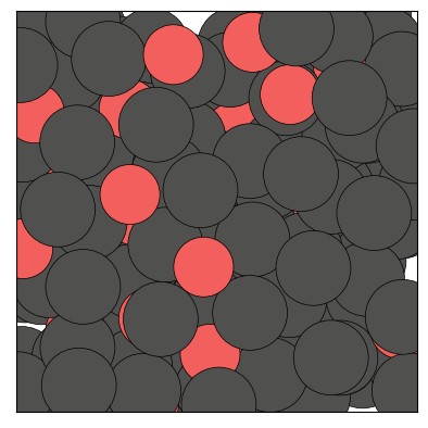
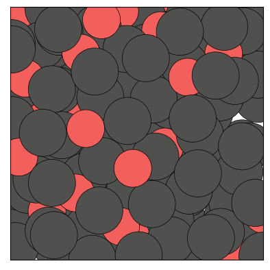
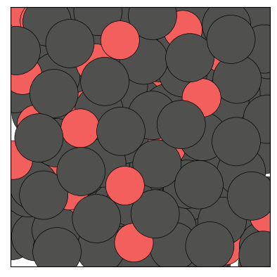
# default coloring code uses the species
figs = traj.show(frames=[0,1,2], backend='matplotlib', show=True)
The Trajectory class being iterable, one can also show a specific frame by calling show() on an element of the trajectory:
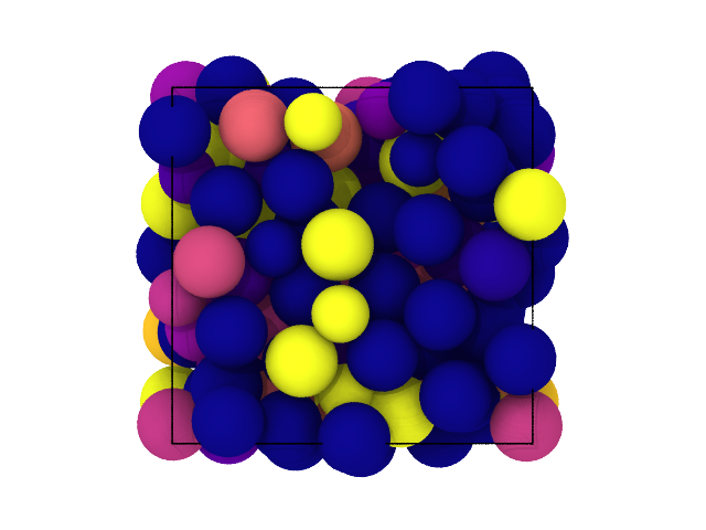
[31]:
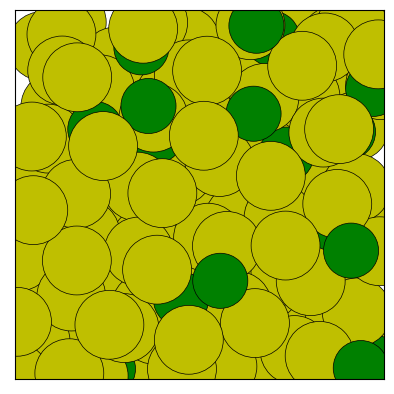
# Show the 5-th frame, change the view, use custom colors
fig = traj[4].show(backend='matplotlib', view='back',
                   palette=['y', 'g'], show=True)
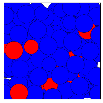
[32]:
# Color particles according to an arbitrary *discrete* particle property
# (for the example, we randomly assign labels to the particles)
traj[0].set_property('label', 0)
p = [0,15,28,37,41,56,63,72,88,90,104,113,125,137,142]
for pi in p:
    traj[0].particle[pi].label = 1
fig = traj[0].show(color='label', palette=['b', 'r'], show=True)
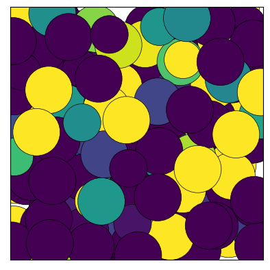
[33]:
from numpy.random import normal

# Color particles according to an arbitrary *continuous* particle property
# (for the example, we randomly assign a random float property to the particles)
rn = [normal() for i in range(150)]
traj[0].set_property('random', rn)
fig = traj[0].show(color='random', cmap='viridis', show=True)
1.8.2. Ovito
See the show_ovito() function in partycls.helpers for more information.
[34]:
from partycls.trajectory import Trajectory

# Open a trajectory file
traj = Trajectory('data/kalj_N150.xyz')
# Adjust radii
traj.set_property('radius', 0.5, "species == 'A'")
traj.set_property('radius', 0.4, "species == 'B'")

# Show the first frame
traj[0].show(backend='ovito')
[34]:
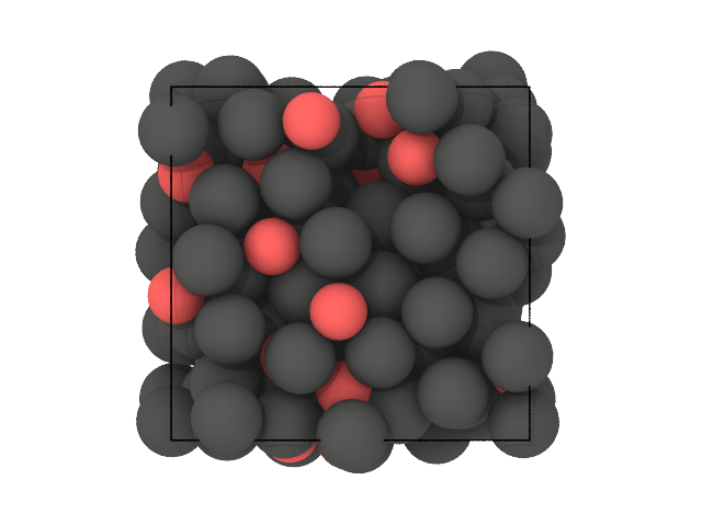
[35]:
# Color particles according to an arbitrary *discrete* particle property
# (for the example, we randomly assign labels to the particles)
traj[0].set_property('label', 0)
p = [0,15,28,37,41,56,63,72,88,90,104,113,125,137,142]
for pi in p:
    traj[0].particle[pi].label = 1

# /!\ Colors must be in RGB format
ovito_colors = [(0.1,0.25,0.9), (0.8,0.15,0.2)]

# Show the first frame
traj[0].show(color='label', backend='ovito', palette=ovito_colors, view='bottom')
[35]:
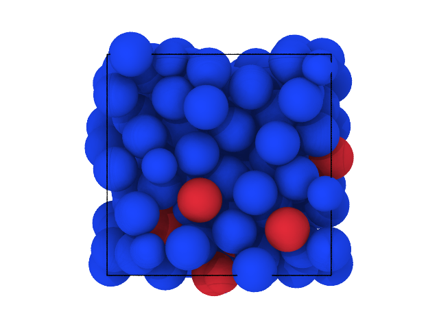
[36]:
from numpy.random import normal

# color particles according to an arbitrary *continuous* particle property
# (for the example, we randomly assign a random float property to the particles)
rn = [normal() for i in range(150)]
traj[0].set_property('random', rn)
traj[0].show(color='random', backend='ovito', cmap='plasma')
[36]:
1.8.3. py3Dmol
See the show_3dmol() function in partycls.helpers for more information.
Warning
This backend works well with small systems, but tends to get pretty slow with larger systems.
[37]:
# Open a trajectory file
traj = Trajectory('data/dislocation.xyz')

# Show the first frame
# Default coloring code uses the species
view = traj[0].show(backend='3dmol')
view.show()
You appear to be running in JupyterLab (or JavaScript failed to load for some other reason). You need to install the 3dmol extension:
jupyter labextension install jupyterlab_3dmol
[38]:
# Color particles according to an arbitrary *discrete* particle property
# (for the example, we randomly assign labels to the particles)
traj[0].set_property('label', 0)
p = [0,5,11,16,20]
for pi in p:
    traj[0].particle[pi].label = 1
view = traj[0].show(backend='3dmol', color='label', palette=['blue', 'red'])
view.show()
You appear to be running in JupyterLab (or JavaScript failed to load for some other reason). You need to install the 3dmol extension:
jupyter labextension install jupyterlab_3dmol
1.9. Writing a trajectory
The class Trajectory can also write a trajectory files with the write() method.
Once the input trajectory has been loaded at the creation of a Trajectory object, any link with the original file is broken: changing the current instance of Trajectory will have no effect on the original file.
Writing a new trajectory file from the current instance can then be useful for many reasons. For example, convert from a format to another:
[39]:
# Open XYZ file
traj = Trajectory('data/traj_with_masses.xyz')

# Write the trajectory in RUMD format (as a new file)
traj.write('data/traj_with_masses.xyz.gz', fmt='rumd')
Or write a trajectory file with additional fields that were not present in the original file:
[40]:
# Open XYZ file
traj = Trajectory('data/traj_with_masses.xyz', additional_fields=['mass'])

# Set custom values for radii of the particles
traj.set_property('radius', 0.5, "species == 'A'")
traj.set_property('radius', 0.4, "species == 'B'")

# Write a new file with both masses and radii
traj.write('data/traj_with_masses_and_radii.xyz', fmt='xyz', additional_fields=['mass', 'radius'])