Tip

Run this notebook online: . Note that the set up can take a while, as all the dependencies must be installed first.

2. Setting and running a workflow

In this notebook, we will see how to perform a streamlined cluster analysis on a trajectory using the Workflow class.

A workflow is a succession of steps to perform a cluster analysis:

1. The computation of a structural descriptor on a given trajectory.

2. An optional feature scaling on the structural features associated to the selected descriptor.

3. An optional dimensionality reduction on the raw/rescaled structural features (depending on step 2.).

4. The execution of a clustering algorithm on the structural features to partition the particles into structurally different clusters.

2.1. The simplest workflow

The Workflow class provides the most straightforward way to perform a spatial clustering of a system.

In its simplest form, this class only requires one positional argument in order to be instantiated: the path to a trajectory file in a supported format or an instance of Trajectory (see the previous notebook for details about trajectories).

Here we analyze a trajectory obtained from the simulation of a Lennard-Jones binary mixture, known as a Kob-Andersen mixture:

from partycls import Workflow

wf = Workflow('data/kalj_N150.xyz')
wf.run()

This is the shortest possible script to run a workflow: we first open a trajectory file through the Workflow class, and use the default parameters to perform each step of the analysis.

Each step can be customized using the following parameters, when instantiating the workflow:

1. descriptor: the type of structural descriptor to use to perform the clustering (see the next notebook and the detailed presentation of each descriptor in the documentation).

   This argument must either be a short string or an instance of StructuralDescriptor (see the partycls.descriptor package). The default value is set to "gr", which is the symbol of the RadialDescriptor class. All compatible string aliases are stored in the class attribute descriptor_db:

print("Available string aliases for descriptors:")
for alias, desc in Workflow.descriptor_db.items():
    print(f'- "{alias}": {desc}')

Available string aliases for descriptors:
- "gr": <class 'partycls.descriptors.radial.RadialDescriptor'>
- "rad": <class 'partycls.descriptors.radial.RadialDescriptor'>
- "radial": <class 'partycls.descriptors.radial.RadialDescriptor'>
- "ba": <class 'partycls.descriptors.ba.BondAngleDescriptor'>
- "ang": <class 'partycls.descriptors.ba.BondAngleDescriptor'>
- "angular": <class 'partycls.descriptors.ba.BondAngleDescriptor'>
- "sbo": <class 'partycls.descriptors.smoothed_bo.SmoothedBondOrientationalDescriptor'>
- "bo": <class 'partycls.descriptors.bo.BondOrientationalDescriptor'>
- "boo": <class 'partycls.descriptors.bo.BondOrientationalDescriptor'>
- "bop": <class 'partycls.descriptors.bo.BondOrientationalDescriptor'>
- "steinhardt": <class 'partycls.descriptors.bo.SteinhardtDescriptor'>
- "labo": <class 'partycls.descriptors.averaged_bo.LocallyAveragedBondOrientationalDescriptor'>
- "ld": <class 'partycls.descriptors.averaged_bo.LechnerDellagoDescriptor'>
- "lechner-dellago": <class 'partycls.descriptors.averaged_bo.LechnerDellagoDescriptor'>
- "lechner dellago": <class 'partycls.descriptors.averaged_bo.LechnerDellagoDescriptor'>
- "sboo": <class 'partycls.descriptors.smoothed_bo.SmoothedBondOrientationalDescriptor'>
- "sbop": <class 'partycls.descriptors.smoothed_bo.SmoothedBondOrientationalDescriptor'>
- "rbo": <class 'partycls.descriptors.radial_bo.RadialBondOrientationalDescriptor'>
- "rboo": <class 'partycls.descriptors.radial_bo.RadialBondOrientationalDescriptor'>
- "rbop": <class 'partycls.descriptors.radial_bo.RadialBondOrientationalDescriptor'>
- "boattini": <class 'partycls.descriptors.radial_bo.BoattiniDescriptor'>
- "tetra": <class 'partycls.descriptors.tetrahedrality.TetrahedralDescriptor'>
- "compact": <class 'partycls.descriptors.compactness.CompactnessDescriptor'>
- "tong-tanaka": <class 'partycls.descriptors.compactness.TongTanakaDescriptor'>
- "tong tanaka": <class 'partycls.descriptors.compactness.TongTanakaDescriptor'>
- "coord": <class 'partycls.descriptors.coordination.CoordinationDescriptor'>
- "coordination": <class 'partycls.descriptors.coordination.CoordinationDescriptor'>

2. scaling: type of feature scaling to apply on the data. Default is None, but a short string (e.g. "zscore" or "minmax") or an instance of the associated classes is also accepted (see the partycls.feature_scaling module). All compatible string aliases are stored in the class attribute scaling_db:

print("Available string aliases for feature scaling:")
for alias, scaling in Workflow.scaling_db.items():
    print(f'- "{alias}": {scaling}')

Available string aliases for feature scaling:
- "standard": <class 'partycls.feature_scaling.ZScore'>
- "zscore": <class 'partycls.feature_scaling.ZScore'>
- "z-score": <class 'partycls.feature_scaling.ZScore'>
- "minmax": <class 'partycls.feature_scaling.MinMax'>
- "min-max": <class 'partycls.feature_scaling.MinMax'>
- "maxabs": <class 'partycls.feature_scaling.MaxAbs'>
- "max-abs": <class 'partycls.feature_scaling.MaxAbs'>
- "robust": <class 'partycls.feature_scaling.Robust'>

3. dim_reduction: dimensionality reduction method. Default value is None, but a short string (e.g. "pca" or "tsne") or an instance of the associated classes is also accepted (see the partycls.dim_reduction module). All compatible string aliases are stored in the class attribute dim_reduction_db:

print("Available string aliases for dim. reduction:")
for alias, redux in Workflow.dim_reduction_db.items():
    print(f'- "{alias}": {redux}')

Available string aliases for dim. reduction:
- "pca": <class 'partycls.dim_reduction.PCA'>
- "tsne": <class 'partycls.dim_reduction.TSNE'>
- "t-sne": <class 'partycls.dim_reduction.TSNE'>
- "lle": <class 'partycls.dim_reduction.LocallyLinearEmbedding'>
- "autoencoder": <class 'partycls.dim_reduction.AutoEncoder'>
- "auto-encoder": <class 'partycls.dim_reduction.AutoEncoder'>
- "ae": <class 'partycls.dim_reduction.AutoEncoder'>

4. clustering: clustering algorithm. Default is "kmeans", but other short strings (e.g. "gmm" or "cinf") or an instance of the associated classes is also accepted (see the partycls.clustering module). All compatible string aliases are stored in the class attribute clustering_db:

print("Available string aliases for dim. reduction:")
for alias, cls in Workflow.clustering_db.items():
    print(f'- "{alias}": {cls}')

Available string aliases for dim. reduction:
- "k-means": <class 'partycls.clustering.KMeans'>
- "kmeans": <class 'partycls.clustering.KMeans'>
- "gaussian mixture": <class 'partycls.clustering.GaussianMixture'>
- "gaussian-mixture": <class 'partycls.clustering.GaussianMixture'>
- "gmm": <class 'partycls.clustering.GaussianMixture'>
- "gm": <class 'partycls.clustering.GaussianMixture'>
- "community inference": <class 'partycls.clustering.CommunityInference'>
- "community-inference": <class 'partycls.clustering.CommunityInference'>
- "inference": <class 'partycls.clustering.CommunityInference'>
- "cinf": <class 'partycls.clustering.CommunityInference'>

In summary, with the three lines of code in cell [1], we used the radial distribution of the particles to form clusters using the K-Means algorithm (no feature scaling or dimensionality reduction by default).

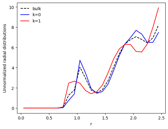
Let us now have a look at the bulk unnormalized radial distribution, and the distributions restricted to the clusters:

import matplotlib.pyplot as plt

# Grid and average distribution
r = wf.descriptor.grid
p_r = wf.descriptor.average

# Dataset: all the individual radial distributions of the particles
data = wf.descriptor.features
# Distributions of the clusters
pk_r = wf.clustering.centroids(data)

# Plot
plt.plot(r, p_r, c='k', ls='--', label='bulk')
plt.plot(r, pk_r[0], c='b', label='k=0')
plt.plot(r, pk_r[1], c='r', label='k=1')
plt.xlabel('r')
plt.ylabel('Unnormalized radial distributions')
plt.legend(frameon=False)
plt.show()

Notes

• descriptor.average refers to the average feature vector of all the samples (i.e. particles) in the dataset. In this example, this is the average radial distribution of the particles.

• clustering.centroids are the coordinates of the cluster centers for the dataset data. This is the average feature vector of all the samples that belong to this cluster. In this example, the average radial distribution of the clusters.

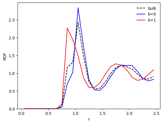
We see that the bulk distribution (dashed line) has been split into two distinctive distributions. Let us have a look at a more common quantity: the radial distribution function (RDF), \(g(r)\).

The class RadialDescriptor, which is the default descriptor used here, implements a normalization method normalize() that allows for two types of normalizations specified by a parameter method:

• method='r2' returns \(r^2g(r)\) (default) ;

• method='gr' returns the standard \(g(r)\) ;

Let us look at the standard \(g(r)\):

# Normalized g(r)
g_r = wf.descriptor.normalize(p_r, method='gr')
g0_r = wf.descriptor.normalize(pk_r[0], method='gr')
g1_r = wf.descriptor.normalize(pk_r[1], method='gr')

# Plot normalized g(r)
plt.plot(r, g_r, c='k', ls='--', label='bulk')
plt.plot(r, g0_r, c='b', label='k=0')
plt.plot(r, g1_r, c='r', label='k=1')
plt.xlabel('r')
plt.ylabel('RDF')
plt.ylim(bottom=0)
plt.legend(frameon=False)
plt.show()

The numbers, fractions and labels of the clusters are accessible through the following attributes:

print('Populations:', wf.populations)
print('Fractions;', wf.fractions)
print('Labels:', wf.labels)

Populations: [10591  4559]
Fractions; [0.69907591 0.30092409]
Labels: [0 0 0 ... 1 1 1]

2.2. Output files

Unless disabled with the wf.disable_output() method, a set output files is written once the cluster analysis is complete. Some are written by default while some need to be enabled. The available output files are:

• "trajectory": a trajectory file with an additional column for the clusters’ labels (if the output format allows it).

• "log": a log file with all the relevant information about the cluster analysis.

• "centroids": a data file with the centroids of the clusters, using the raw features from the descriptor.

• "labels": a text file with the clusters’ labels only.

• "dataset": a data file with the raw features from the descriptor.

All the information regarding output files is stored in the instance attribute output_metadata (dictionary):

# All possible types output files
print(wf.output_metadata.keys())

dict_keys(['trajectory', 'log', 'centroids', 'labels', 'dataset'])

Each of these files has its specific options. For instance, the options for the output trajectory file are:

# Options for the output trajectory
print("All options:\n", wf.output_metadata['trajectory'].keys())

# Default values of some options
print('\nEnable output:', wf.output_metadata['trajectory']['enable'])
print('\nOutput format:', wf.output_metadata['trajectory']['fmt'])

All options:
 dict_keys(['enable', 'writer', 'filename', 'fmt', 'backend', 'additional_fields', 'precision'])

Enable output: True

Output format: xyz

Output metadata can be changed through the method set_output_metadata(). For instance:

wf.set_output_metadata('trajectory',
                       filename='my_traj.xyz.gz',
                       fmt='rumd')

If no filename is provided for the output files, a default naming convention will be used.

The default naming convention of every file is defined by the attribute wf.naming_convention:

print(wf.naming_convention)

{filename}.{code}.{descriptor}.{clustering}

Each tag in the previous string will be replaced by its value in the current instance of Worfklow. This naming convention can be changed by using any combination of the following tags:

• {filename}: name of the input trajectory file.

• {code}: extension for files produced by partycls.

• {descriptor}: descriptor used.

• {scaling}: feature scaling method used.

• {dim_reduction}: dimensionality reduction method used.

• {clustering}: clustering method used.

In our example, setting

wf.naming_convention = "{filename}_{clustering}_{descriptor}"

would create output files with the following names:

• kalj_N150.xyz_kmeans_gr.log.

• kalj_N150.xyz_kmeans_gr.dataset.

• Etc.

2.3. A customized workflow

Let us now look at a more complex example, where the Workflow is fully customized.

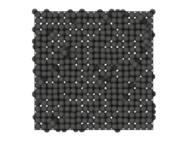
We consider a cubic crystal in which some particles have been dislocated from their original lattice positions:

from partycls import Trajectory

# Load the trajectory
xtal_traj = Trajectory('data/dislocation_N8000.xyz')

# Visualize the first (and only) frame
xtal_traj[0].show(backend='ovito')

We use simple angular correlations, a standard feature scaling method (Z-score) and a linear dimensionality reduction technique (PCA) to find the clusters:

from partycls.descriptors import BondAngleDescriptor
from partycls import PCA

# Bond-angle descriptor
D_ba = BondAngleDescriptor(xtal_traj)
X = D_ba.compute()

# Dimensionality reduction method
redux = PCA(n_components=2)

# Workflow
xtal_wf = Workflow(xtal_traj,
                   descriptor=D_ba,
                   scaling='zscore',
                   dim_reduction=redux,
                   clustering='kmeans')
xtal_wf.clustering.n_init = 100 # clustering repetitions
xtal_wf.run()

Note

The raw features, rescaled features, and features in the reduced space are accesible through the attributes features, scaled_features and reduced_features respectively.

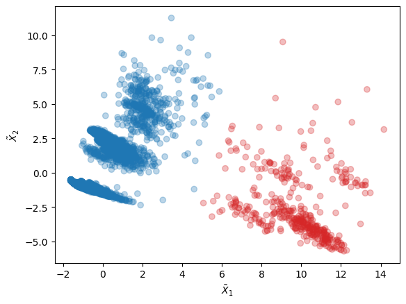
Let us look at the clusters in the 2D latent space corresponding to the two principal components the PCA instance with largest eigenvalues:

import numpy as np

# Features in latent space and labels
X_red = xtal_wf.reduced_features
labels = xtal_wf.labels

# Scatter plot of latent space with clusters' labels
c = np.array(['tab:blue', 'tab:red'])
plt.scatter(X_red[:,0], X_red[:,1], c=c[labels], alpha=0.3)
plt.xlabel(r"$\tilde{X}_1$")
plt.ylabel(r"$\tilde{X}_2$")
plt.show()

We now look at the centroids of the clusters (i.e. bond-angle distributions in our example):

# Grid and centroids
theta = D_ba.grid
C_k = xtal_wf.clustering.centroids(X)

# Make centroids normalized bond angle distributions
q_0 = D_ba.normalize(C_k[0], method='pdf')
q_1 = D_ba.normalize(C_k[1], method='pdf')

# Bond-angle distributions
plt.plot(theta, q_0, c='tab:blue', label='k=0')
plt.plot(theta, q_1, c='tab:red', label='k=1')
plt.legend(frameon=False)
plt.xlabel('Bond-angle, ' + r'$\theta$' + ' (deg.)')
plt.ylabel('Bond-angle distribution, ' + r'$q(\theta)$')
plt.ylim(bottom=0)
plt.show()

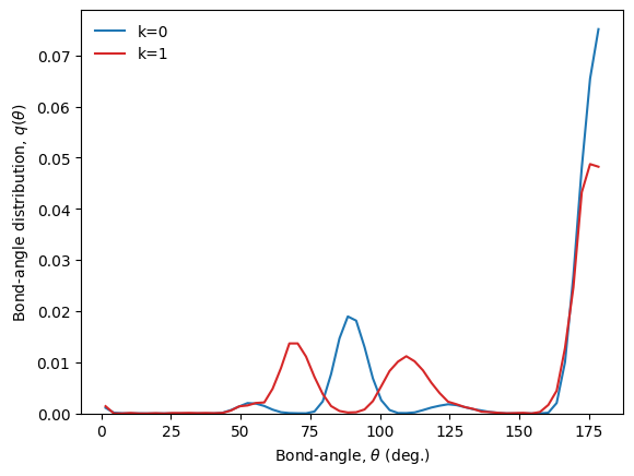
This is what is expected: particles on the lattice dislocated particles belong to two different clusters.

We can verify this by looking at the clusters directly in real-space:

# Show the system with labels
xtal_traj[0].show(backend='ovito', color='label', palette=[(0,0,1), (1,0,0)])

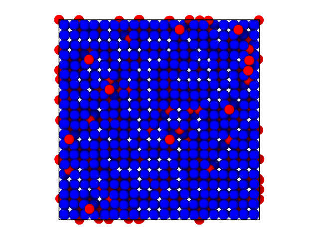
Dislocated particles are colored differently from the crystal, as expected.